WpProj:
Linear p-Wasserstein Projections![]()
The goal of WpProj is to perform Wasserstein projections
from the predictive distributions of any model into the space of
predictive distributions of linear models. This package employs the
methods as described in Eric
Dunipace and Lorenzo Trippa (2020). <arXiv:2012.09999>.
The Wasserstein distance is a measure of distance between two probability distributions. It is defined as
\[W_p(\mu,\nu) = \left(\inf_{\pi \in \Pi(\mu,\nu)} \int_{\mathbb{R}^d \times \mathbb{R}^d} \|x-y\|^p d\pi(x,y)\right)^{1/p}\]
where \(\Pi(\mu,\nu)\) is the set of all joint distributions with marginals \(\mu\) and \(\nu\).
In the our package, if \(\mu\) is the original prediction from the original model, such as from a Bayesian linear regression or a neural network, then we seek to find a new prediction \(\nu\) that minimizes the Wasserstein distance between the two,
\[\mathop{\text{argmin}} _ {\nu} W _ {p}(\mu,\nu) ^ {p},\]
subject to the constraint that \(\nu\) is a linear model.
To reduce the complexity of the number of parameters, we add an L1 penalty to the coefficients of the linear model to reduce the complexity of the model space,
\[\mathop{\text{argmin}} _ {\nu} W _ {p}(\mu,\nu) ^ {p} + P_{\lambda}(\nu),\]
where \(P_\lambda(\nu)\) is a penalty on the complexity of the model space such as the the \(L_1\) penalty on the coefficients of the linear model.
You can install the development version of WpProj from GitHub with:
# install.packages("devtools")
devtools::install_github("ericdunipace/WpProj")This is a basic example running the WpProj function on a
simulated dataset. Note we create a pseudo posterior from a simple
dataset for illustration purposes:
library(WpProj)
set.seed(23048)
# note we don't generate believable data with real posteriors
# these examples are just to show how to use the function
n <- 32
p <- 10
s <- 21

# covariates and coefficients
x <- matrix( stats::rnorm( p * n ), nrow = n, ncol = p )
beta <- (1:10)/10

#outcome
y <- x %*% beta + stats::rnorm(n)

# fake posterior
post_beta <- matrix(beta, nrow=p, ncol=s) + stats::rnorm(p*s, 0, 0.1)
post_mu <- x %*% post_beta #posterior predictive distributions

# fit models
## L1 model
fit.p2     <-  WpProj(X=x, eta=post_mu, power = 2.0,
                   method = "L1", #default
                   solver = "lasso" #default
)

## approximate binary program
fit.p2.bp <-  WpProj(X=x, eta=post_mu, theta = post_beta, power = 2.0,
                   method = "binary program",
                   solver = "lasso"
                   # this is the default because
                   # the approximate algorithm is faster
)
We can compare the performance of the models using the
distCompare function (measuring distance between the
reduced models and the original model) and then generate a plot
dc <- distCompare(models = list("L1" = fit.p2, "Binary Program" = fit.p2.bp),
                  target = list(parameters = post_beta,
                                  predictions = post_mu))
p <- plot(dc, ylabs = c("2-Wasserstein Distance", "2-Wasserstein Distance"))
p$parameters + ggplot2::ggtitle("Parameters")
p$predictions + ggplot2::ggtitle("Predictions")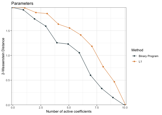
We can also compare performacne by measure the relative distance between a null model and the predictions of interest as a pseudo \(R^2\)
r2.null  <- WPR2(projected_model = dc) # should be between 0 and 1
plot(r2.null)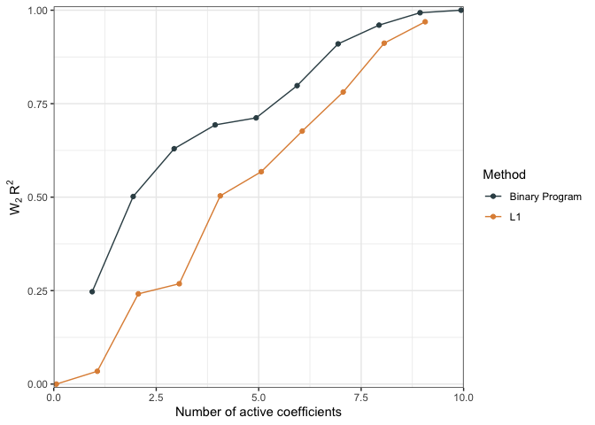
We can also examine how the predictions change in the models as more covariates are added for individual observations.
ridgePlot(fit.p2, index = 21, minCoef = 0, maxCoef = 10)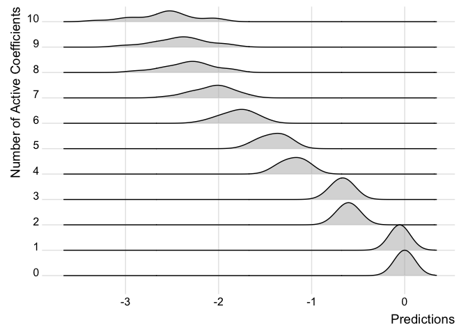
Note how the predictions get better the more coefficients are added and the distribution looks closer to the full posterior predictive.
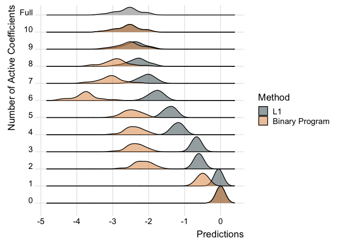
We can also compare the two models like so:
ridgePlot(list("L1" = fit.p2, "Binary Program" = fit.p2.bp), index = 21, minCoef = 0, maxCoef = 10, full = post_mu[21,])